

Building a powerful soil spectroscopy model is a significant achievement, but its true utility and reliability hinge on rigorous validation of soil spectroscopy model lab reference data. Without proper validation, even sophisticated models remain unproven hypotheses, potentially leading to costly field mistakes.
Many promising models fail in real-world applications due to insufficient validation. This process isn’t just about achieving good numbers; it’s about building trust in predictions for farmers and agronomists. Robust spectroscopy model validation ensures consistently accurate, actionable insights from new soil samples.
The core idea is simple: prove your model works reliably on unseen data. This article outlines essential steps and considerations for effectively validating soil spectroscopy models, bridging laboratory precision with practical field application. We’ll cover techniques and metrics to build confidence in your predictive capabilities.
Why Validation Is as Important as Model Building
Many optimize algorithms but rush validation – a critical error. A model performing well on training data but poorly on new data is useless for precision agriculture. Proper spectroscopy model validation reveals if your model learns general patterns or merely memorizes training examples.
Inaccurate nutrient predictions can lead to over-fertilization (wasting money, harming the environment) or under-fertilization (reduced yields). These real-world consequences underscore the need to rigorously validate soil spectroscopy model lab reference data, safeguarding against faulty insights.
Validation provides an unbiased estimate of your model’s predictive performance on unseen data, crucial for production. Without it, you operate on assumptions, not proven capabilities. This process helps manage expectations and communicate your technology’s actual reliability to stakeholders.
Overfitting occurs when a model becomes too complex, capturing noise instead of underlying relationships. A strong validation strategy immediately exposes overfitting, prompting simplification or collection of more diverse training data. Aim for a model that generalizes well, not one that merely scores high on familiar samples.
Validation also objectively compares modeling approaches. With multiple algorithms or preprocessing techniques, a consistent framework helps determine which method offers the best predictive power, shifting focus from theoretical elegance to practical effectiveness in precision agriculture.

Validation is an integral part of the model development lifecycle, influencing every decision from data collection to algorithm selection. This iterative approach ensures your final model is robust, reliable, and ready for real-world deployment.
Ignoring proper validation risks significant financial losses and reputational damage. Inaccurate recommendations quickly erode trust, hindering future technology adoption. Investing in thorough spectroscopy model validation establishes credibility and fosters long-term success in precision agriculture.
Key Statistics: RMSECV, RMSEP, RPD, and Bias Explained Simply
To validate soil spectroscopy model lab reference data, concrete metrics are essential. Root Mean Square Error of Cross-Validation (RMSECV) and Root Mean Square Error of Prediction (RMSEP) are fundamental statistics. RMSECV measures internal cross-validation performance, while RMSEP assesses it on an independent validation set.
The Ratio of Performance to Deviation (RPD) normalizes model quality, showing predictive power against natural data variation. Bias indicates consistent over- or under-prediction. Together, these metrics provide a comprehensive picture of your model’s accuracy and reliability, highlighting strengths and weaknesses.
| Statistic | What It Measures | Ideal Value | Interpretation |
|---|---|---|---|
| RMSECV | Model error during internal cross-validation | Lower is better | Error on data seen during model training |
| RMSEP | Model error on independent validation data | Lower is better | True predictive error on unseen data |
| RPD | Ratio of standard deviation to RMSEP | Higher is better (>2.5 for good prediction) | Model’s ability to predict against natural variation |
| Bias | Systematic over- or under-prediction | Close to zero | Indicates consistent deviation from actual values |
| R² (Coefficient of Determination) | Proportion of variance explained by model | Closer to 1 is better | How well predictions fit actual values |
Designing an Independent Validation Set That Avoids Overfitting
Creating a truly independent validation set is critical for preventing overfitting and ensuring model generalization. This set must comprise soil samples entirely excluded from model training and initial calibration. You cannot simply use a random subset from your original dataset if it contributed to model development.
I advocate collecting new, geographically diverse samples specifically for validation, ideally from different seasons or management practices than the training data. This tests your model against the full spectrum of real-world variability, truly validating soil spectroscopy model lab reference data and building trust.
A common mistake is random data splitting without considering spatial or temporal correlations. If samples from the same field or time are split between training and validation, the set isn’t truly independent. The model might perform well by memorizing similar samples, not by learning robust general patterns.
To mitigate this, use a “hold-out” strategy: reserve an entire field, region, or year of data exclusively for validation. This ensures the model faces genuinely new conditions, providing a more honest assessment of its predictive power and yielding reliable results.
The size of your independent validation set is significant. It must be large enough to be statistically representative of the target population. Too few samples can lead to an unreliable RMSEP, hindering firm conclusions about model performance.
Ensure the validation set covers the full range of soil properties and environmental conditions in your target area. If your model is for diverse soil types, the validation set must reflect this. A narrow set only confirms performance within that range, risking poor predictions elsewhere.
I recommend collecting validation samples from challenging or unusual soil areas. If your model performs well on these “edge cases,” confidence in its robustness increases significantly. This strategic data collection is a cornerstone of effective spectroscopy model validation.
Leave-One-Out vs. K-Fold Cross-Validation: Which to Use
Cross-validation assesses model performance and selects optimal parameters without an independent validation set during initial development. It estimates how well your model generalizes to unseen data by systematically partitioning training data, crucial for robust model development before final independent validation.
Leave-One-Out Cross-Validation (LOOCV) and K-Fold Cross-Validation are common methods. Each has advantages and disadvantages, with the choice depending on dataset size and computational resources. Understanding these differences informs your spectroscopy model validation strategy.
Leave-One-Out Cross-Validation (LOOCV) trains the model on all but one sample, then tests on that single sample, repeating for every dataset sample. While providing a nearly unbiased performance estimate, its computational cost is prohibitive for large soil spectroscopy datasets, especially during rapid iteration. This often makes LOOCV impractical.
K-Fold Cross-Validation divides the dataset into ‘k’ equal-sized folds. The model trains on k-1 folds and validates on the remaining fold, repeating ‘k’ times so each fold serves as the validation set once. This significantly reduces computational burden compared to LOOCV, while still providing a robust performance estimate.
Common choices for ‘k’ include 5 or 10, balancing bias and variance. Higher ‘k’ means more training data per fold, potentially leading to a less biased performance estimate but increased computation. Lower ‘k’ is faster but might yield a more biased estimate, making the choice crucial for spectroscopy model validation.
I generally prefer K-Fold Cross-Validation for its efficiency and reliability, especially with large soil spectroscopy datasets. It offers a stable RMSECV estimate without LOOCV’s prohibitive computational demands. The choice of ‘k’ should be justified by dataset size and validation goals.
When implementing K-Fold, ensure each fold maintains the same distribution of target variables as the full dataset, especially with stratified sampling. This prevents unrepresentative folds from skewing RMSECV results. Careful partitioning ensures a fair assessment of your model’s internal consistency.
Both methods aim to provide a reliable estimate of model performance on unseen data. However, K-Fold is often more practical for real-world soil spectroscopy applications. Remember, cross-validation is an internal process; the final test must always be against a truly independent validation set to comprehensively validate soil spectroscopy model lab reference data.
Interpreting Residual Plots to Diagnose Model Weaknesses
Beyond numerical statistics like RMSEP and RPD, residual plots offer invaluable insights into model performance and weaknesses. A residual plot graphs the difference between predicted and actual lab reference values. This visual representation helps diagnose systematic errors that statistical metrics might obscure, deepening your understanding of spectroscopy model validation.
Ideally, a residual plot shows a random scattering of points around zero, indicating random, unbiased errors across predictions. Any discernible pattern signals an underlying model or data problem. Interpreting these patterns is a crucial skill for model developers to fine-tune their approach.
- Funnel Shape: Indicates heteroscedasticity; error increases with predicted value.
- Curved Pattern: Suggests a non-linear relationship not captured by the model.
- Outliers: Points far from the main cluster, possibly data entry errors or unique samples.
- Banded Pattern: Could indicate categorical variables not properly handled.
- Shifted Mean: Consistent positive or negative residuals, showing bias in predictions.
When to Accept a Model and When to Rebuild From Scratch
Deciding whether to accept or rebuild a model is a judgment call guided by objective criteria and application requirements. A model is acceptable when its RMSEP and RPD values meet predefined thresholds for your precision agriculture task, often determined by the economic impact of prediction errors.
If RMSEP is too high or RPD too low (e.g., below 2.0), your model is likely inaccurate for practical use. Consistently reliable predictions are needed, not just occasional correctness. Such a model fails to adequately validate soil spectroscopy model lab reference data for real-world application, requiring further work.
Beyond primary statistics, examine prediction bias. Consistent positive or negative bias suggests a systematic error needing address, even with a reasonable RMSEP. This could indicate issues with calibration standards or systematic differences between spectroscopy and lab data. Aim for an accurate and unbiased model across its prediction range.
Residual plots are also significant. Clear patterns like a funnel shape or curve indicate missing crucial information or relationships. Ignoring these visual cues means deploying a model with known weaknesses, a recipe for field failure.
Sometimes, the issue lies not with the model, but with training data quality or representativeness. If training data lacks diversity or fails to cover the target environment’s full variability, even optimal algorithms will struggle to generalize. Rebuilding then means collecting more comprehensive, targeted soil samples, not just tweaking algorithms.
The hardest decision can be scrapping a heavily invested model. However, clinging to a mediocre model due to sunk cost fallacy is unproductive. Rebuilding with a refined data collection strategy or different modeling approach often yields superior results, prioritizing robust performance over past effort.
Consider the practical implications of model errors. An error in predicting soil pH might be less critical than one in phosphorus, depending on crop and regulations. Aligning acceptance criteria with real-world impact enables pragmatic deployment decisions, essential for effective spectroscopy model validation.
If your model performs well overall but struggles with specific soil types, consider developing specialized sub-models instead of a single global model. This acknowledges soil science complexity, allowing tailored, accurate predictions in specific contexts, significantly improving overall system performance.
Documenting Validation Results for Reproducibility and Reporting
Thorough documentation of validation results is as crucial as the validation itself, ensuring reproducibility and transparent reporting. This means detailing every step, from independent validation set creation to specific metrics calculated, not just noting the final RMSEP. Without it, results are difficult to verify or replicate.
Clearly describe the independent validation dataset: its size, geographical origin, collection methods, and unique characteristics. This context is essential for understanding your model’s validated performance scope and limitations, providing sufficient detail for others to trust your claims and the basis of your spectroscopy model validation.
Meticulously record all performance metrics: RMSEP, RPD, R², and bias, with confidence intervals if applicable. Presenting these in tables and figures (e.g., residual plots, scatter plots of predicted vs. actual values) conveys information effectively, making complex data easier to interpret.
Detail the exact software, algorithms, and parameters used for model building and validation. Version control for code and data is non-negotiable for reproducibility. Documentation should enable others, given the same data, to replicate your exact validation results, building trust with users and collaborators.
Always include a discussion of validation challenges: outliers, missing data, or unexpected residual patterns. Acknowledging limitations and areas for improvement adds credibility. No model is perfect; transparently addressing weaknesses demonstrates a mature understanding of its capabilities.
For stakeholders, summarize key findings in clear, non-technical language, focusing on practical implications. Translate RMSEP and RPD into real-world terms, explaining the error range for precision agriculture decisions. This ensures everyone, regardless of technical background, understands the model’s reliability.
Maintain a version history of validation reports, especially as models update or new data emerges. This audit trail is invaluable for tracking improvements, diagnosing regressions, and demonstrating continuous development, reinforcing the reliability of your soil analysis system.
Finally, consider peer review or external auditing, particularly for high-stakes applications. Independent assessment catches overlooked issues, strengthening model credibility. This external scrutiny powerfully validates soil spectroscopy model lab reference data and ensures its fitness for purpose.
A well-documented validation process forms the bedrock of scientific integrity in precision agriculture. It confirms your model is a transparent, verifiable tool, not a black box. This commitment ensures spectroscopy model validation withstands scrutiny and serves as a reliable asset for agricultural decision-making.
Ultimately, documenting validation results reflects confidence in your model’s ability to deliver accurate, actionable insights. This confidence, backed by rigorous data, drives successful adoption and meaningful impact in agriculture, setting a standard for reliability and precision benefiting all involved.
Validating soil spectroscopy models against lab reference data is a fundamental commitment to accuracy and reliability in precision agriculture, not just a technical exercise. Validation quality directly impacts farmer trust and decision efficacy. Rigorous protocols ensure your models are truly fit for purpose.
From designing independent validation sets to interpreting residual plots, every step builds a robust, trustworthy system. A model’s true value lies not in complexity, but in its proven ability to deliver accurate real-world predictions. This dedication to validation differentiates your solutions in a competitive market.