

Understanding soil properties through spectroscopy offers immense potential for precision agriculture. However, raw spectral data often contains noise and unwanted variations that can obscure the true chemical information we seek. This is where spectral pre-processing becomes a critical step in developing accurate predictive models.
Ignoring these preliminary steps is like trying to read a blurry document; you might get the gist, but you will miss crucial details. Effective spectral pre-processing helps isolate the signal of interest from various interferences, making the data more interpretable and robust for analysis. We need methods to clean up the spectral signature before we can truly understand it.
This article will explain key spectral pre-processing techniques, including scatter correction and baseline removal, which are essential for soil spectroscopy. We will look into how these methods address common issues in spectral data and ultimately improve the performance of your predictive models. Properly cleaned data paves the way for reliable insights in soil mineralogy and beyond.
Why Raw Spectra Need Pre-Processing Before Modeling
Raw spectral data, especially from soil samples, rarely arrives ready for immediate modeling. Several physical and environmental factors introduce unwanted variations that are unrelated to the chemical composition we aim to measure. These interferences can compromise accuracy and reliability of subsequent statistical analysis.
Particle size differences within soil samples are a major culprit, causing light scattering that distorts the spectral signal. Variations in sample moisture content also absorb light differently, complicating spectral interpretation. These physical characteristics mask the subtle absorbance bands we are actually trying to observe.
Beyond sample properties, instrument drift and ambient light fluctuations can also introduce systemic errors. These instrumental artifacts create inconsistencies across measurements, making it difficult to compare samples or replicate results. Accounting for these issues is fundamental to good experimental practice.
Without proper spectral pre-processing, a predictive model might learn irrelevant variations instead of actual chemical relationships. This leads to models that perform poorly on new, unseen data, which is a significant problem in precision agriculture. You want your model to understand the soil, not the noise.
Therefore, applying appropriate pre-processing techniques is a necessary step for building robust and accurate spectroscopic models. It ensures your model focuses on true chemical information, leading to more reliable predictions of soil properties. This careful preparation is the foundation for successful soil spectroscopy.
Understanding Multiplicative Scatter Correction (MSC)
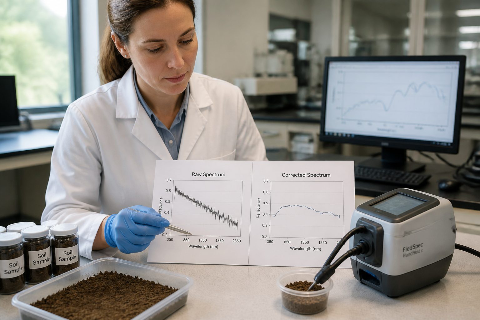
Multiplicative Scatter Correction (MSC) is a widely used spectral pre-processing technique designed to compensate for scattering effects in diffuse reflectance spectra. These scattering effects primarily arise from particle size and packing density differences. MSC aims to normalize baseline and intensity variations across your spectral dataset.
The core idea behind MSC is to correct each spectrum by comparing it against a reference spectrum, often the mean spectrum. It corrects baseline shifts by subtracting the regression line’s intercept, then adjusts for slope differences multiplicatively. This method effectively reduces physical light scattering on your soil spectroscopy results.
| MSC Step | Description | Impact on Spectra |
|---|---|---|
| Mean Spectrum Calculation | Averaging all individual spectra in the dataset to create a reference. | Establishes a common “target” for correction, representing the average scattering profile. |
| Linear Regression | Fitting a linear model for each individual spectrum against the mean spectrum. | Determines the baseline offset (intercept) and intensity scaling (slope) for each sample. |
| Baseline Correction | Subtracting the intercept of the regression line from each individual spectrum. | Aligns the baseline of all spectra, removing additive variations. |
| Intensity Correction | Dividing the baseline-corrected spectrum by the slope of the regression line. | Normalizes the intensity differences, reducing multiplicative scattering effects. |
MSC is particularly effective for NIR scatter correction in soil samples, where particle size variations influence light interaction. By minimizing these physical variations, MSC enhances underlying chemical absorption features. This makes it easier for models to identify and quantify soil constituents.
Proper application of MSC can improve the signal-to-noise ratio and consistency of your spectral data. This leads to more robust and accurate calibration models for soil properties, which is invaluable for precision agriculture. It is a fundamental step in preparing soil spectral data for analysis.
Standard Normal Variate (SNV): When to Use It Instead of MSC
Standard Normal Variate (SNV) is another powerful spectral pre-processing technique addressing scatter and path length variations, similar to MSC. However, SNV operates on each spectrum independently, normalizing it without reference to other spectra. This makes SNV a computationally simpler alternative in many cases.
SNV works by subtracting each spectrum’s mean and dividing by its standard deviation. This process effectively centers and scales each spectrum, removing both multiplicative and additive effects. It’s a quick way to achieve scatter correction.
While MSC uses a global reference (the mean spectrum of the dataset), SNV uses an internal reference (each spectrum’s mean and standard deviation). This distinction means SNV can be particularly useful when a representative mean spectrum is difficult to obtain or with highly diverse datasets. It offers spectrum-by-spectrum normalization.
Researchers often debate using MSC, SNV, or both for soil spectroscopy. Generally, if your dataset has a consistent spectral pattern and you expect similar scattering across samples, MSC might provide a more harmonized correction. If your samples are highly heterogeneous or processing spectra individually, SNV can be more practical.
Both MSC and SNV reduce baseline shifts and intensity variations from scattering, but their mechanics differ. Choice depends on your soil spectral data characteristics and analysis objectives. It is often beneficial to test both and compare their impact on model performance.
Ultimately, the goal is to make chemical information more prominent by minimizing physical noise. SNV provides a robust way to achieve this, making it a valuable tool in spectral pre-processing for soil analysis. Its independent operation can sometimes prevent the propagation of errors from a poorly chosen reference spectrum.
Baseline Correction Methods: Detrending and First Derivatives
Beyond scatter correction, baseline variations obscure analytical signals in spectral data. These variations often arise from background absorbance, instrument drift, or sample matrix effects, shifting the spectrum. Effective spectral baseline correction is essential for accurate peak identification and quantification.
Detrending is a straightforward baseline correction method that involves fitting and subtracting a polynomial function from the spectrum’s baseline. This removes slow-varying background signals, flattening the baseline and making absorption peaks more prominent. It is a simple yet powerful.
The order of the polynomial used for detrending is a critical parameter; a first-order polynomial removes linear trends, higher orders correct complex curvatures. Choosing the correct order prevents over-correction, which could remove valuable chemical information. You want to flatten the baseline without distorting the peaks.
First derivative transformation is another powerful baseline correction method that removes baseline shifts and resolves overlapping peaks. This technique calculates the rate of change of absorbance with respect to wavelength, transforming peaks into derivative shapes. It makes subtle spectral changes more noticeable.
Applying a first derivative eliminates constant and linearly sloping baselines. This enhances resolution of closely spaced peaks and often improves calibration curve linearity. However, it also amplifies noise, so smoothing often precedes derivative calculation.
Both detrending and derivative methods are forms of spectral pre-processing that aim to isolate true chemical absorption features from unwanted background signals. The choice depends on baseline issues and whether overlapping peaks need resolution. Combining techniques often yields best results for complex soil spectra.
Understanding these baseline correction methods is fundamental to achieving high-quality spectral data for soil analysis. They ensure models interpret actual chemical changes rather than instrumental or physical artifacts. Clean baselines are a sign of well-prepared data.
Smoothing Techniques: Savitzky-Golay and Its Parameters
Spectral data often contains random noise, from instrument electronics or environmental fluctuations. This noise can obscure subtle spectral features and reduce predictive model accuracy. Smoothing techniques are employed in spectral pre-processing to reduce random noise without distorting the signal.
The Savitzky-Golay (SG) filter is one of the most popular and effective smoothing algorithms in spectroscopy. It works by fitting a low-degree polynomial to a small window of data points and replacing the central point with the polynomial’s value. This local polynomial fitting preserves peak shape and height better than moving average filters.
- Window Size: Number of data points used for polynomial fitting.
- Polynomial Order: Degree of the polynomial fitted within the window.
- Number of Passes: How many times the filter is applied.
- Derivative Order: Simultaneously calculate derivatives during smoothing.
- Symmetry: Whether the window is centered or asymmetric.
Choosing the right Savitzky-Golay filter parameters is crucial. A larger window size provides more smoothing but can broaden peaks and reduce resolution if too large. A higher polynomial order retains more signal shape but might not smooth noise effectively if the window is too small.
Often, the SG filter is used with derivative calculations, performing both smoothing and differentiation in a single step. This combination is powerful for spectral pre-processing, simultaneously reducing noise and enhancing subtle spectral features. It streamlines data preparation.
The key is to find a balance where noise is reduced without significant distortion or loss of spectral information. Experimentation with window sizes and polynomial orders is usually necessary for optimal settings in soil spectroscopy data. Visual inspection of the smoothed spectra is always a good practice.
Proper smoothing is an integral component of a comprehensive spectral pre-processing strategy. It prepares data for subsequent steps like baseline correction or modeling, ensuring clear chemical signals. A well-smoothed spectrum provides a much better foundation for accurate predictions.
Choosing the Right Pre-Processing Combination for Your Data
Selecting the optimal combination of spectral pre-processing techniques is rarely one-size-fits-all; it depends on your soil spectral data characteristics and study objectives. There is no universally “best” approach, making careful consideration and experimentation essential. You need to understand your data’s unique challenges.
Start by visually inspecting raw spectra to identify issues like baseline shifts, varying intensities, and noise. Are baselines drifting significantly, suggesting a need for spectral baseline correction? Are there clear differences in overall signal intensity, pointing towards scatter correction methods like MSC or SNV?
Sequential application of techniques often yields the best results. For example, applying scatter correction (MSC or SNV) first normalizes overall intensity, followed by a smoothing filter (Savitzky-Golay) to reduce random noise. After these steps, baseline correction (detrending or derivative) can further refine spectral features. The order matters for cumulative effect.
Consider your target soil property; some properties are more sensitive to certain noise or baseline variations. For instance, properties identified by subtle peak shifts might benefit more from derivative transformations. Understanding the chemistry helps guide the pre-processing choices.
A common strategy involves testing several pre-processing combinations and evaluating their impact on model performance. Use metrics like R-squared, RMSE, or RPD from cross-validation to assess which combination leads to the most accurate and robust predictions. This empirical approach is often most reliable.
Remember that over-processing can be as detrimental as under-processing, potentially removing valuable information or introducing artifacts. It is a delicate balance between cleaning data and preserving its chemical integrity. Always monitor spectral changes during each pre-processing step to ensure no signal loss.
Documenting pre-processing choices and parameters is crucial for reproducibility and transparency. This allows replication of findings and ensures consistency in future analyses. Good documentation is part of good scientific practice in soil spectroscopy.
How Pre-Processing Choices Affect Final Model Performance
The decisions made during spectral pre-processing have a profound and direct impact on the performance, robustness, and interpretability of final predictive models. These initial data transformations are not cosmetic; they fundamentally alter how a model perceives underlying relationships. It is a foundational stage for model success.
Incorrect or insufficient spectral pre-processing can lead to models that overfit to noise or irrelevant variations, resulting in poor generalization. Such models might show high training accuracy but fail dramatically in real-world precision agriculture. This is a common pitfall for new practitioners.
For instance, failing to apply effective NIR scatter correction means models might interpret particle size differences as chemical variations. This leads to biased predictions inconsistent across samples with varying physical characteristics. The model learns the physics of light interaction rather than the chemistry of the soil.
Similarly, neglecting spectral baseline correction can cause models to struggle with distinguishing true absorption peaks from broad background shifts. This reduces model sensitivity to chemical constituents, making accurate quantification difficult. A flat baseline helps the model focus on the meaningful peaks.
On the other hand, appropriate pre-processing, such as MSC, SNV, or well-tuned smoothing, enhances the signal-to-noise ratio and standardizes spectral features. This allows the model to better identify and learn true chemical correlations. The model becomes more intelligent about the data.
Improved data quality from effective pre-processing translates into higher R-squared values, lower RMSE, and better predictive accuracy. These improvements are critical for developing reliable tools for nutrient management, soil health assessment, and precision agriculture applications. Better models mean better decisions.
Ultimately, investing time in understanding and applying the right spectral pre-processing techniques is an investment in the quality and utility of spectroscopic models. It is a non-negotiable step that differentiates mediocre from highly effective models. This careful attention to detail truly pays off in the end.
Optimizing Pre-Processing for Specific Soil Properties
The ideal spectral pre-processing strategy often varies depending on the specific soil property to predict. Different soil constituents exhibit unique spectral signatures and are influenced differently by physical interferences. Therefore, a generic approach might not always yield the best results for every target variable.
For properties heavily influenced by organic matter (e.g., total carbon or nitrogen), prioritize pre-processing that enhances broad NIR absorption features. This could involve careful baseline correction to remove interfering water absorption bands. The goal is to isolate the specific chemical signals associated with these compounds.
When predicting soil texture properties (e.g., clay or sand content), scattering effects are prominent due to particle size variations. In these cases, robust NIR scatter correction methods like MSC or SNV are essential to normalize spectral intensity. These methods help the model focus on the compositional differences rather than just particle size.
Trace elements or specific mineral phases often present subtle absorption features easily masked by noise or overlapping signals. For these challenging predictions, derivative transformations, possibly combined with advanced smoothing, can help resolve and emphasize these weak bands. The sensitivity of these methods is key.
Moisture content is another significant factor in soil spectroscopy; its strong absorption bands can overshadow other chemical signals. When predicting other properties in variable moisture conditions, pre-processing might include specific water removal algorithms or careful selection of spectral regions less affected by water. You need to account for this dominant interference.
Developing an optimized spectral pre-processing workflow often involves an iterative process of trial and error, combined with a deep understanding of soil chemistry and spectroscopy. It is about tailoring the approach to unique challenges presented by each soil property and its spectral manifestation. This customized approach maximizes predictive accuracy.
By consciously selecting and fine-tuning pre-processing steps based on the target soil property significantly enhances predictive power. This targeted optimization is a hallmark of advanced soil spectroscopy for precision agriculture. It moves beyond generic cleaning to intelligent data preparation.
Challenges and Best Practices in Spectral Pre-Processing
Despite clear benefits, spectral pre-processing has challenges; understanding them helps avoid pitfalls. One major hurdle is over-processing, where excessive filtering or transformation can remove valuable chemical information. This can lead to less accurate or interpretable models.
Another challenge is noise amplification, particularly with derivative transformations, making subtle features harder to discern. While smoothing helps, balancing noise reduction and signal preservation requires careful parameter tuning. It is a constant trade-off in spectral pre-processing.
A key best practice involves visualizing spectra at each pre-processing stage. This visual inspection helps understand each step’s impact and identify if valuable information is distorted or lost. Trust your eyes as much as your statistical metrics.
Furthermore, apply the exact same pre-processing steps to both calibration and validation datasets. Inconsistency introduces significant bias, rendering model performance metrics unreliable. This ensures fair comparison and accurate evaluation of model generalization ability.
Consider external validation sets, independent of calibration data, to rigorously test your chosen pre-processing strategy’s robustness. If the model performs well on an external set, it suggests pre-processing effectively handles real-world sample variations. This is the ultimate test of your methods.
Documenting your entire pre-processing workflow, including algorithms and parameter settings, is a non-negotiable best practice. This ensures reproducibility and allows for easy iteration and improvement in future analyses. Good record-keeping is vital for scientific rigor.
Finally, experiment with different combinations of spectral pre-processing techniques. The optimal solution is often found through systematic testing and comparison. This iterative process is part of becoming proficient in soil spectroscopy.
Embracing these best practices helps overcome challenges and maximizes the effectiveness of spectral pre-processing efforts. This leads to more reliable and impactful models for precision agriculture. It is about smart data management from start to finish.
Spectral pre-processing is an indispensable stage from raw spectral data to actionable insights in precision agriculture. Techniques like scatter correction, including MSC and SNV, effectively address physical variations obscuring chemical information. Meanwhile, detrending and first derivatives tackle baseline shifts and enhance peak resolution, crucial for accurate analysis.
Smoothing algorithms, especially the Savitzky-Golay filter, play a vital role in reducing random noise, ensuring subtle chemical signals are not lost. The careful selection and combination of these pre-processing steps directly influence predictive model performance and reliability. It is a foundational element for robust soil spectroscopy.
By dedicating attention to proper spectral pre-processing empowers models to accurately interpret soil properties, leading to more informed field decisions. This commitment to data quality translates into more efficient resource management and sustainable agricultural practices. It truly unlocks the full potential of soil spectroscopy.